Origins of Life: Building a Hypercycle Simulation with WebGL

Though the exact origins of life on earth remain a mystery, there are a number of tools we can use to try to understand and explain the emergence of self-replicating systems, a key pre-requisite. One of the most interesting models is the hypercycle, which describes a set of cyclical chemical reactions which together form self-replicating loops of emergent behaviors.

These self-replicating loops represent a plausible model of the origin of life.  Also, they look pretty freakin' cool. In this post, we'll explore what a hypercycle is, how it can teach us about the origins of life, and how we can build a hypercycle simulation using WebGL pixel shaders.

What is a "Hypercycle"?

A hypercycle is a mathematical model that describes a set of chemical reactions, leading to a cycle of molecules that depend on each other for their survival. Each molecule in the hypercycle catalyzes the replication of another molecule in the system, forming a cycle of replication that is self-sustaining.

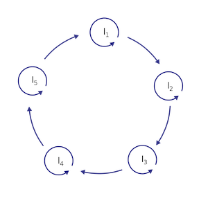
Self-replication is the ability of a molecule or system to make copies of itself: a process that is essential for the emergence of life. In a hypercycle, each molecule catalyzes the replication of another molecule in the system, creating a cycle of self-replication.

If we introduce a spatial element into the model, we can simulate the hypercycle in a reaction-diffusion system.  Reaction-diffusion systems describe the behavior of chemicals that interact with each other through chemical reactions and are transported through a medium by diffusion. These systems can create complex patterns and behaviors that are essential to the formation of life.

What can the Hypercycle teach us about the origins of life?

The hypercycle is a simple model for explaining the emergence of self-replicating systems. The model proposes that the first self-replicating systems on earth were sets of molecules that catalyzed each other's replication, forming a self-sustaining cycle of replication.  This interdependence creates a selection pressure that favors the evolution and adaptation of the system as a whole.  Over time, the theory goes, these self-replicating systems evolved and adapted, eventually giving rise to the first living cells.

It's worth noting that the hypercycle is an abstract model.  Generally speaking, the model does not propose a specific set of chemicals or reactions.  Instead, it's simply a model which lets us probe some of the properties that could give rise to such self-replicating systems.  In principle, hypercycle behavior can emerge from simple chemical reactions, RNA molecules,  proteins  or even entire organisms (of the three options, the "RNA world" hypothesis is the most popular).

So while the model doesn't predict the exact agents involved in the origin of life on earth, we can use simulation of hypercycles to explore all kinds of questions related to the origins of self-replication and life:

• What kinds of networks of chemical reactions can form self-replicating systems?
• What kinds of temporospatial dynamics give rise to stable populations?
• What are the effects of changing variables like reactivity and diffusion rates
• What other kinds of changes to the system (like temperature, introduction of other agents), can stabilize or destabilize self-replicating hypercycles?

In short, while it doesn't predict a specific set of agents or behaviors responsible for the origin of life, it can help us understand the conditions under which self-replication and life can emerge.

How do we build a Hypercycle simulation?

To build a hypercycle simulation, we need to understand the math behind the hypercycle.  The hypercycle can be described mathematically as a set of differential equations that describe the replication of each molecule in the system. These equations can be solved numerically to simulate the behavior of the system over time.

Formally, the hypercycle equations are defined as:

At each timestep, the chemical x_i is produced through a reaction with chemical x_j at a rate specified by k_i,j.  In most models, each chemical i reacts only with i-1, so this can be simplified–the summation term is replaced with a single reaction term.  k_i represents the rate of self-reproduction and degradation of a chemical itself (and can sometimes be ignored).   The φ term at the end is a degradation expression based on the concentration of all of the chemicals, which keeps the total concentration constant.

Additionally, to satisfy the cyclical nature of the model, we assume that the "first" and "last" chemical x refer to the same entity:

Things get really interesting when we introduce a spatial dynamic as well.  The math is similar, but occurs at every point on a huge grid.  Additionally, the chemicals spread out or diffuse slightly at each time step.  

To simulate and visualize the hypercycle, we'll build a discretized version of the reaction-diffusion system with spatial dynamics using OpenGL shaders in order to  create a realistic real-time simulation of a hypercycle.  Our strategy will be to create a texture that represents the spatial concentration of the chemicals at each pixel.  We'll use the standard 4 color channels (red, green, blue and alpha) to represent the concentrations of 4 different chemicals which comprise the hypercycle.  

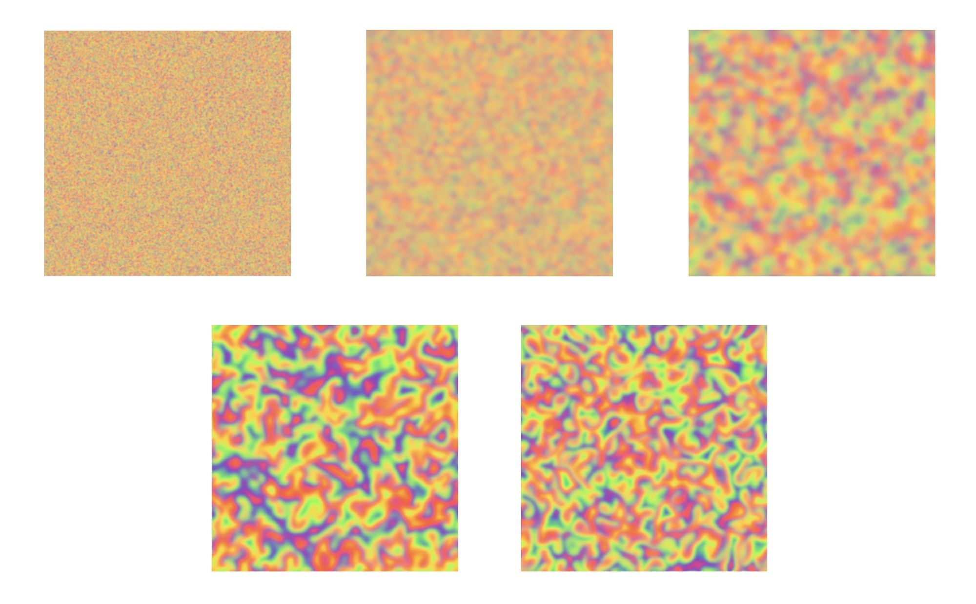
Before getting into the details, here's a demo of our model that you can inspect and play with.  You can make changes to the model, or adjust the reaction, diffusion and decay constants to see what kinds of effect it has on the behavior of the system.

You can play with the model, including adjusting the core reaction and diffusion parameter values to see what effects it has on the system as a whole.  By modifying those values, we can create different kinds of visual patterns, transition the system from stable to chaotic dynamics  or "blow up" the simulation completely.

The Hypercycle Simulation in WebGL

To build our interactive hypcercycle simulation, we'll create a couple of simple pixel shaders in WebGL.  We use a simple wrapper called SwissGL to help us setup the WebGL environment and execute the shaders.  In this post we show only the shader code itself – if you wish to see the full code used to setup and execute the shaders, you can find it in the Codepen example above.

Our simulation is made up of three simple shader programs: one to initialize the data, one to perform our simulation at each timestep, and the last to display our simulation data on screen.  

First, we have a simple shader to initialize our data to some pseudo-random values.  This shader could be almost anything that produces initial data (including an existing image texture), but in this case, we use SwissGL's built-in random hash function to sample random data based on a seed we provide:

vec4 random = vec4(
  hash(ivec3(I, seed * 1.0)).x,
  hash(ivec3(I, seed * 2.0)).x,
  hash(ivec3(I, seed * 3.0)).x,
  hash(ivec3(I, seed * 4.0)).x
);
out0 = normalize(random);

The output of this shader is stored in a texture that represents the state of our system.

Next is the core simulation loop.  At each step, we compute the next state by taking the current state, then calculating and combining terms for reaction, diffusion and decay, and storing the results in an updated state texture:

precision highp float;

// Diffusion: sample a pixel in each direction, scale by diffusionRate 
vec4 current = texture(points, UV);
float dx = 1.0 / size;
vec4 n1 = texture(points, UV + vec2(dx, 0));
vec4 n2 = texture(points, UV + vec2(0, dx));
vec4 n3 = texture(points, UV + vec2(-dx, 0));
vec4 n4 = texture(points, UV + vec2(0, -dx));
vec4 diffusion = diffusionRate * (((n1 + n2 + n3 + n4) / 4.0) - current);

// Reaction: chemical x reacts with (x-1) scaled by reactionRate:
vec4 reaction = (reactionRate * current * current.argb);

// Decay: chemicals decay at decayRate (can be 0)
vec4 decay = current * (1.0 - decayRate);

// Output: sum our terms and normalize
out0 = normalize(decay + reaction + diffusion);

Note that our reaction term uses pixel swizzling to multiple each chemical concentration by the previous chemical concentration.  This is the "cycle" part of our simulation:  current.rgba * current.argb .

Finally, with the simulation state updated, we can display the state of our simulation on screen.  Though we could sample the simulation state texture directly and use the result as the color value to display, it doesn't always produce the best results.  Instead, we'll assign a color to each chemical in the simulation, and produce a final color value weighted by the concentrations of each chemical:

vec4 s = texture(points, UV);
vec3 color = (s.x * c1 + s.y * c2 + s.z * c3 + s.w * c4);
out0 = vec4(color, 1.0);

Probing the Origins of Life – In Software

The hypercycle model provides an intriguing framework for understanding the origins of self-replicating systems and the emergence of life on earth.  By studying the behavior of self-replicating systems, we can gain insight into the fundamental principles that govern the behavior of living systems.

The hypercycle is just one example of how mathematical models and computer simulations can help us better understand the real world, and in some cases, help us explore the mysteries and origins of life itself.